MLE and MAP

One most common situation is, we have a model that could produce the (unnormalized) probability \( p(x|\theta) \) for some observation \( x \). We are often interested in the most probable \( \theta \) given the data, i.e. \( \theta^* = \arg\max_\theta p(\theta|x) \).

Applying the Bayes’ rule, \( \theta^* = \arg\max_\theta p(x|\theta)p(\theta)/p(x). \) Since \( p(x) \) is independent of \( \theta \), it doesn’t affect the outcome of the \( \arg\max \) operation, we got \( \theta^* = \arg\max_\theta p(x|\theta)p(\theta) \), which is known as maximum a posteriori (MAP). If we assume a uniform (uninformative) prior \( p(\theta) \), if can be further reduced to just \( \theta^* = \arg\max_\theta p(x|\theta) \), which is known as maximum likelihood estimation (MLE).

Bayesian Methods

Sometimes we care more about the entire posterior distribution \( p(\theta|x) \) rather than a point estimation (\( \arg\max \)), in which case \(\theta\) is treated as a (latent) random variable insteand of a parameter.

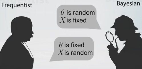
These two approaches (point estimation and posterior distribution) are derived from the Frequentist v.s. Bayesian views of Statistics respectively. There’s a neat introduction on Coursera, Bayesian approach to statistics.

Posterior Probability

The difficulty of Bayesian methods often arises in computing the marginal \( p(x) = \int p(x|\theta)p(\theta) d\theta \), as mentioned in Pattern Recognition and Machine Learning

In the case of continuous variables, the required integrations may not have closed-form analytical solutions, while the dimensionality of the space and the complexity of the integrand may prohibit numerical integration. For discrete variables, the marginalizations involve summing over all possible configurations of the hidden variables, and though this is always possible in principle, we often find in practice that there may be exponentially many hidden states so that exact calculation is prohibitively expensive.

Ideally we would like \( p(\theta) \) to be the conjugate prior of the likelihood function \( p(x|\theta) \), so that the posterior can be solved analytically and furthermore can be used again as the prior for subsequent analyses. For instance say the model follows \( N(x|f(\theta), \sigma) \), and the prior of \( \theta \) is also Gaussian, then the posterior would be another Gaussian distribution if \( f(\theta) \) is linear.

Conjugate prior-likelihood pairs often allow the marginal \( p(x) \) to be expressed in closed form. In other cases we normally turn to variational methods or sampling or the combination of both for approximation.

Discussion

Do not be confused with the notion of the discriminative and generative models. In discriminative (\( p(y|x) \)) and generative (\( p(y, x) \)) models, it assumes the data can be formed as \(x\) the input and \(y\) the target. While in our discussion, \(x\) is the data \(\theta\) is the parameter, how we solve for the parameters is independent of which model we choose.