Introduction

Naive Bayes and logistic regression are two basic machine learning models that are compared frequently, especially as the generative/discriminative counterpart of one another. However at first sight it seems these two methods are rather different. In naive Bayes we just count the frequencies of features and labels while in linear regression we optimize the parameters with regard to some loss function. If we express theses two models as probabilistic graphical models, we’ll see exactly how they are related.

Graphical Models

naive Bayes
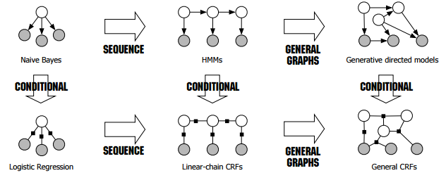
As shown in the figure (borrowed from this tutorial without permission), the naive Bayes model can be expressed as a directed graph where the parent node denotes the output and the leaf nodes denote the input, the joint probability is then \[p(x, y)=p(y)\prod_n p(x_i|y).\]

logistic regression
The logistic regression model can be expressed as the conditional counterpart of the naive Bayes model. \[\tilde{p}(x, y)=\psi(y)\prod_n\psi(x_i, y)\] \[p(y|x)=\frac{1}{z(x)}\tilde{p}(x, y)\] \[z(x)=\sum_y\tilde{p}(x, y).\]

To have the network structure and parameterization correspond naturally to a conditional distribution, we want to avoid representing a probabilistic model over x. We therefore disallow potentials that involve only variables in x. –Probabilistic Graphical Models

Maximum Likelihood Estimation (MLE)

In the simplest case where both the input and output are binary values, for the naive Bayes model, both \(p(y)\) and \(p(x_n|y)\) can be modeled as Bernoulli distributions \[p(y)=Ber(y|\theta_0)\] \[p(x_i|y)=Ber(x_i|\theta_{yi})\] \[p(y=1|x)=\frac{\theta_0\prod \theta_{1i}^{x_i}(1-\theta_{1i})^{1-x_i}}{\theta_0\prod \theta_{1i}^{x_i}(1-\theta_{1i})^{1-x_i}+(1-\theta_0)\prod \theta_{0i}^{x_i}(1-\theta_{0i})^{1-x_i}}.\] Then the MLE for \(\theta\) could simply be solved by counting the frequencies.

For the logistic regression model, we can choose the log-linear representation with feature functions as the followings \[\psi(x_i, y)=\exp(w_i\phi(x_i, y))=\exp(w_i I(x_i=1, y=1))\] \[\psi(y)=\exp(w_0\phi(y))=\exp(w_0 y)\] then it follows \[\tilde{p}(x, y=1)=\exp(\sum_n w_ix_i+w_0)\] \[\tilde{p}(x, y=0)=\exp(\sum_n w_i\times 0+w_0\times 0)=1\] \[p(y=1|x)=\frac{\tilde{p}(x, y=1)}{\tilde{p}(x, y=1)+\tilde{p}(x, y=0)}=\sigma(\sum_n w_ix_i+w_0)\] \[p(y|x)=Ber(y|\sigma(\sum_n w_ix_i+w_0)).\] The MLE for \(w\) can be done by minimizing the negative log-likelihood (a.k.a cross-entropy).

In this example, the number of effective parameters in \(w\) is fewer than \(\theta\) as it only models the conditional probability (we can always only parameterize n-1 out of n categories then the probability of the remaining category can be inferred as they sum up to one).

Overfitting and Zero Probabilities

The most common problem for MLE is overfitting, for naive Bayes it can lead to zero probabilities for unseen data. Smoothing techniques are often used to mitigate this, which can be interpreted as a prior assumption.

Conditional Independence

Logistic regression is consistent with the naive Bayes assumption that the input \(x_i\) are conditionally independent given \(Y\). Nevertheless unlike NB (which models every \(p(x_i|y)\) separately), LR only optimizes for the conditional likelihood, it has better performance than NB when the data disobeys the assumption (e.g. when two features are highly correlated).