Markov Chains

By Markov chains we refer to discrete-time homogeneous Markov chains in this blog.

A discrete-time Markov chain is a sequence of random variables \({X_1, X_2, X_3, …}\) with the Markov property, namely that the probability of moving to the next state depends only on the present state and not on the previous states \[p(X_{n+1}|X_n,…,X1) = p(X_{n+1}|X_n).\]

A homogeneous Markov chain is one that does not evolve in time, that is, its transition probabilities are independent of the time step \(n\) \[p(X_{n+1}|X_n) \text{ is same } \forall n \leq 0.\]

Water Lily Example

To illustrate we’ll take a look at the water lily example from this Bayesian Methods for Machine Learning course on coursera.

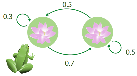
There a frog in a pond that jumps between two water lilies following some probability. As shown in the graph, if the frog is at the left lily at time \(n\) then it has 0.7 probability to jump to the right lily and 0.3 probability to stay till the next time \(n+1\), if the frog is at the right lily then probability for staying and jumping are even (0.5).

This process can be modeled as a Markov chain, let \(X_n\in\{L, R\}\) be the state of the frog at time \(n\), we have the transition probabilities \[p(X_{n+1}=L|X_n=L)=0.3, p(X_{n+1}=R|X_n=L)=0.7\] \[p(X_{n+1}=L|X_n=R)=0.5, p(X_{n+1}=R|X_n=R)=0.5.\]

If we let the frog jump as described for a long enough period, it turns out the probability of the state of the frog will converge to a fixed distribution \(\pi\) regardless of the starting state, specifically \(\pi(X=L)=0.44\), \(\pi(X=R)=0.56\). It is an interesting property of Markov chains and we’ll spend the rest of this blog on discussing relevant concepts and applications.

Stationary Distribution

For a Markov chain, if a distribution \(\pi\) remains unchanged through time it is called a stationary distribution, formally it follows \[\pi(X_{n+1}=i)=\sum_j\pi(X_{n}=j)p(X_{n+1}=i|X_{n}=j).\]

If there’s a finite number of possible states in the sample space, this condition can be put in matrix form as \[\pi=\pi P\] where \(P_{ij}=p(X_{n+1}=i|X_{n}=j)\). It might look similar to the definition of eigenvalues and eigenvectors \[Av=\lambda v\] In fact \(\pi\) is an eigenvector of \(P^T\) (a.k.a a left eigenvector of \(P\)) with eigenvalue \(\lambda=1\) \[(P^T-I)\pi=0\] \(\pi\) is called a vector in the null space of \(P^T-I\) by definition. So to find the stationary distribution of a finite state Markov chain, we only need to solve the above system of linear equations.

One commonly raised issue here is, in what case there is one and only one stationary distribution (one and only one \(\lambda=1\))?

Closed Communicating Classes (Irreducible Closed Subsets)

Following the definition on Wikipedia

• A state \(j\) is said to be accessible from a state \(i\) if a system started in state \(i\) has a non-zero probability of transitioning into state \(j\) at some point.
• A state \(i\) is said to communicate with state \(j\) if both \(i\) is accessible from \(j\) and vice versa. A communicating class is a maximal set of states \(C\) such that every pair of states in \(C\) communicates with each other.
• A communicating class is closed if the probability of leaving the class is zero. Having defined the notion of a closed communicating class, now we can use it to find out the number of stationary distributions.

For finite state Markov chains, it can be shown that every transition matrix has, at least, an eigenvector associated to the eigenvalue 1 and the largest absolute value of all its eigenvalues is also 1. Hence we know every finite state Markov chain has at least one stationary distribution.

If there’s one closed communicating class in the chain, the chain has exactly one stationary distribution. For example in the following transition matrix, \[ \begin{matrix} 0.5 & 0 \
0.5 & 1 \
\end{matrix} \] there’s one closed communicating class consisting of only one state \(C=\{1\}\), and \(\pi=[0, 1]\) is the unique stationary vector. If there’s more than one closed communicating classes, then there are infinitely many stationary distributions. For example the identity matrix \[ \begin{matrix} 1 & 0 \
0 & 1 \
\end{matrix} \] each of the two states itself is a closed communicating classes, in this case any probability vector is stationary \(\pi I=\pi \).

For infinite state Markov chains, the states in closed classes has to be positive recurrent for stationary distributions to exist (for finite chains we get the positive recurrence within closed classes for free), otherwise there are no stationary distributions.

Here are lecture notes from M3S4/M4S4 Applied Probability (Imperial College), tutorial by Karl Sigman and this question for reference.

Irreducibility

If the entire state space forms one closed communicating class, then the chain is called irreducible.

PageRank

The famous PageRank algorithm is an application of the Markov chain stationary distribution. Each web page can be think of as a state, links to other pages then represent the transition probabilities to other states, and each link on a page is considered equally probable.

Having the states and transition probabilities defined, the process of a person randomly clicking on links can be modeled by such Markov chain. The PageRank algorithm ranks pages according to the stationary probability, which can be interpreted as the probability of arriving at a page through random clicking.

As one can imagine the transition matrix can be very sparse as the number of links on a page is far less than the total number of pages. To ensure that there’s a unique stationary distribution, we can add a [teleportation probability to the matrix to make all entries strictly positive, as described in here (Lecture 33: Markov Chains Continued Further, Statistics 110) and here (How Google Finds Your Needle in the Web’s Haystack). It’s obvious that a stochastic matrix with strictly positive entries is irreducible, hence there’s a unique stationary distribution.

Limiting Distribution

Now we know a Markov chain has a unique stationary distribution \(\pi\) if there’s one closed positive recurrent communicating class, one may wonder how does a Markov chain behave as \(n\to\infty\).

There are two limiting behaviours people usually care about. The first is whether the sample average converges to the stationary distribution as \(n\to\infty\) \[\lim_{n\to\infty} \frac{1}{n} \sum^{n}_{m=1} I\{X_m=i\}=\pi_i \text{ w.p.1}\] where \(X_m \sim p(X_m|X_0)\) are samples from the Markov chain (ref: this tutorial by Karl Sigman).

Second if the state distribution always converges to the stationary distribution for any initial probability \(X_0\), then \(\pi\) is called the limiting distribution \[\pi = \lim_{n\to\infty} p(X_n|X_0). \] Clearly, a limiting distribution is always a stationary distribution and a Markov chain can have only one limiting distribution.

Let’s illustrate the difference between these two behaviours by an example. The matrix \[ \begin{matrix} 0 & 1 \
1 & 0 \
\end{matrix} \] has only one eigenvector \(\pi=[0.5, 0.5]\) associated to the eigenvalue 1. Say a frog start at the left lily, in the next step it will jump to the right lily w.p.1 according to the matrix, after another step, it will again jump to the left and so forth like this video shows :))

Actually it will alternate between two states periodically and never reaches a stationary distribution. Nevertheless if we draw two samples at a time, they can be thought of as samples from the stationary distribution as the average of two alternating distributions from this chain is the stationary distribution, so the sample average converges to the expectation w.r.t. the stationary distribution.

It turns out convergence without averaging is a stronger condition than convergence with averaging, to go from the first to the second, a further condition known as aperiodicity is needed for the chain. Discussion about how to check the first property can be found here, a commonly used sufficient condition is irreducible + positive recurrent.

Ergodicity

Another commonly mentioned property is called ergodicity, which is essentially having a limiting distribution while being irreducible, more specifically,

• for a finite MC it holds that, aperiodic + irreducible (which implies positive recurrent) ⇔ ergodic
• for an infinite MC it holds that, aperiodic + irreducible + positive recurrent ⇔ ergodic
  for more detail of these different properties you can take a look at 18.2, 18.3, 18.4 and 18.5 of the ML video series by mathematicalmonk, and this tutorial by Yuri Suhov.

KL Divergence

It is shown in the book Elements of Information Theory 2nd (Section 4.4) that for any state distributions \(p\) and \(q\), a Markov chain will bring them closer together (at least no further away) step after step in terms of KL divergence \[D_{KL}(p_n|q_n)\geq D_{KL}(p_{n+1}|q_{n+1})\] If \(q\) is a stationary distribution, we have \[D_{KL}(p_n|\pi)\geq D_{KL}(p_{n+1}|\pi)\] which implies that any state distribution gets no further away to every stationary distribution as time passes. The sequence \(D_{KL}(p_n|\pi)\) is a monotonically non-increasing non-negative sequence and must therefore have a limit. The limit is always zero for limiting distributions.

In the previous example, the state distribution alternates between \([1,0]\) and \([0,1]\) the KL divergence \(D_{KL}(p_n|\pi)\), though not increasing, remains \(\log 2\).

The Second Eigenvalue

We know a Markov chain will converge to its limiting distribution from any state if there’s one, so when will it converge? For finite state Markov chains, the convergence speed depends on the second large eigenvalue in magnitude of the transition matrix.

A sloppy sketch of the proof goes as follows. Assume for simplicity that all eigenvalues of the transition matrix \(P\) are real and distinct. Then it can be decomposed as \(P = V\Lambda V^{-1}\), where \(\Lambda\) is a diagonal matrix of eigenvalues, \(V\) is a matrix of right eigenvectors and \(V^{-1}\) is a matrix of left eigenvectors, we know \(P^n =V\Lambda^n V^{-1} \) (ref: Diagonalizing a Matrix). Then we decompose the initial distribution as a linear combination of the left eigenvectors \(X_0=QV^{-1}\) where \(Q\) is a diagonal matrix. The state distribution at time \(n\) is then
\[X_n = X_0P^n =QV^{-1}V\Lambda^nV^{-1} = Q\Lambda^nV^{-1}.\] Since the largest eigenvalue in \(\Lambda\) is one and others have magnitude smaller than \(1\), the rest elements in \(\Lambda^n\) will vanish as \(n\to\infty\). So \(X_n\) will converge to the stationary distribution eigenvector \(\pi\) in \(V^{-1}\), and the difference between \(X_n\) and \(\pi\) is in proportional to \(|\lambda_2|^n\), where \(\lambda_2\) is the second large eigenvalue in magnitude.

For a detailed proof please see Markov Chains and Random Walks on Graphs, and here is a nice animated illustration exponential convergence and the 3x3 pebble game École normale supérieure.

Monte Carlo (Sampling)

Monte Carlo methods were central to the simulations required for the Manhattan Project during the war. The general idea is to estimate expected values using samples, especially when the exact values are hard to compute analytically \[E_p[f(X)]=\int f(X)p(X) dX \approx \frac{1}{M}\sum^M_{m=1}f(X_m)\] where \({X_m}\) are samples from \(p(X)\).

The core problem is how to draw samples from a given distribution and what property should the samples possess. Usually we would want independent samples, while sometimes using correlated samples can be more efficient and accurate in terms of estimating expected values. We’ll illustrate the difference by the following example.

Sampling Wheel (Low Variance Resampling)

For detailed introduction of the sampling wheel (low variance resampling) algorithm please see Particle Filters: The Good, The Bad, The Ugly, we only discuss a simplified version here.

tbc

MCMC

Drawing samples from an arbitrary distribution is not easy, especially on high dimensional space, we’re going to see how to use Markov chains for Monte Carlo estimation a.k.a Markov chain Monte Carlo (MCMC).

The central idea of MCMC is to construct a Markov chain with a unique stationary distribution being the target distribution \(\pi\). Then based on the limiting behaviour of Markov chains \[\lim_{n\to\infty} \frac{1}{n} \sum_{m=1}^{n} I\{X_m=i\}=\pi_i \text{ w.p.1}\]
it can be derived \[E_{\pi}[f(X)] \approx \frac{1}{N}\sum^N_{i=1}f(X_i)\] for any bounded function \(f\).

Further if \(\pi\) is a limiting distribution, \[\pi = \lim_{n\to\infty} P(X_n|X_0) \] then starting from an arbitrary state \(X_0\) then state it’ll be in after the chain converges can be seen as a sample from \(\pi\). Based on these two properties, there are many strategies out there for estimating expected values and drawing (independent) samples, which are not to be discussed in this blog.

We’ve already discussed how to check the existence of a unique stationary distribution and a limiting distribution. Now let’s see how to construct a Markov chain with a given stationary distribution \(\pi\), which at the same time should be easier to draw samples from.

Gibbs Sampling

For some high dimensional distributions, sampling from it’s one dimensional conditional distribution is easy, the Gibbs sampling method makes use of this property by sampling iteratively over each dimension.

Suppose we have a three dimensional distribution \(p(X1, X2, X3)\), and we’re in state \((X1_{n}, X2_{n}, X3_{n})\) at time \(n\), we get to the next state following the strategy \[X1_{n+1}\sim p(X1|X2_n, X3_n) \] \[X2_{n+1}\sim p(X2|X1_{n+1}, X3_n) \] \[X3_{n+1}\sim p(X3|X1_{n+1}, X2_{n+1}). \] The transition probability is then \[p(X1_{n+1}, X2_{n+1}, X3_{n+1}|X1_n, X2_n, X3_n) = p(X1|X2_n,X3_n) p(X2|X1_{n+1},X3_n) p(X3|X1_{n+1},X2_{n+1}). \] It’s easy to show that \(p(X1, X2, X3)\) is a stationary distribution of the Markov chain constructed (see this lecture).

Metropolis Hastings

Detailed Balance \[\pi(X_{n}=i)p(X_{n+1}=j|X_{n}=i)=\pi(X_{n}=j)p(X_{n+1}=i|X_{n}=j) \forall i,j \] is a sufficient but not necessary condition for a distribution to be stationary. Still sampling directly form \(\pi\) is hard, unlike Gibbs sampling, where the transition probability is separated into one dimensional conditional probabilities, the Metropolis Hastings algorithm decomposes the transition probability into a proposal distribution \(q\) (easy to sample from) and an acceptance factor \(\alpha\) (to satisfy detailed balance). Say at time \(n\) we’re in state \(x_n\), then we draw a sample \(x_{n+1}’\) from the proposal distribution \(q(X_{n+1}|X_{n})\) and then accept it with probability \(\alpha(X_{n+1}, X_{n})\), if accepted, we move to the sampled stated, otherwise we remain at the same state. Thus the transition probability becomes \[p(X_{n+1}=j|X_{n}=i) = q(X_{n+1}=j|X_{n}=i)\alpha(X_{n+1}=j,X_{n}=i) \text{ for } i\neq j\] \[p(X_{n+1}=i|X_{n}=i) = q(X_{n+1}=i|X_{n}=i)\alpha(X_{n+1}=i,X_{n}=i) + \sum_{j}q(X_{n+1}=j|X_{n}=i)(1-\alpha(X_{n+1}=j,X_{n}=i))\]

The acceptance probability \(\alpha\) need to satisfy \[\frac{\alpha(X_{n+1}=j,X_{n}=i)}{\alpha(X_{n+1}=i,X_{n}=j)}=\frac{\pi(X_{n}=j)q(X_{n+1}=i|X_{n}=j)}{\pi(X_{n}=i)q(X_{n+1}=j|X_{n}=i)}.\] Meanwhile its value has to be between 0 and 1, one solution could be \[\alpha(X_{n+1}=j,X_{n}=i)=\min (1, \frac{\pi(X_{n}=j)q(X_{n+1}=i|X_{n}=j)}{\pi(X_{n}=i)q(X_{n+1}=j|X_{n}=i)} ).\] Since target distribution \(\pi\) only appears as a ratio, it allows \(\pi\) to be an unnormalized distribution. This is very helpful when the normalizer is hard to compute.

It may seem a bit weird that there’s a large probability to remain at the same state at every move because of the acceptance probability. Actually self loops will affect the speed of convergence, but they won’t change the stationary distribution as long as detailed balance is satisfied, it’s analogous to the fact that adding a constant to all diagonal elements of a matrix doesn’t change the eigenvectors.

Discussions

Markov Chain Stationary Distribution Problem