Summary of Latent Dirichlet Allocation

What does LDA do?

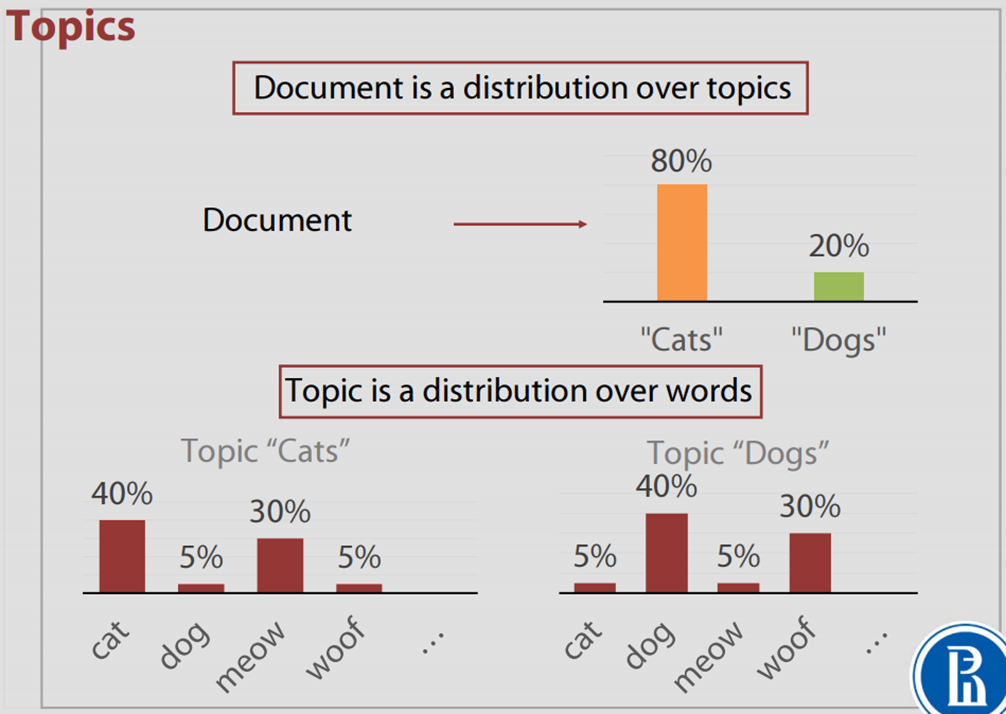
The LDA model converts a bag-of-words document in to a (sparse) vector, where each dimension corresponds to a topic, and topics are learned to capture statistical relations of words. Here’s a nice illustration from Bayesian Methods for Machine Learning by National Research University Higher School of Economics. lda

LDA vs. vector space model

The vector space model representation of a document is a normalized vector in the “word” space, while the LDA representation is a normalized vector in the “topic” space. By converting a bag-of-words document from a “word” space into a “topic” space, we can incorporate word correlations learned under the topics.

History

The LDA paper gives a good summary of the history of text modeling.
Unigram model
\[p(\mathbf{w})=\prod_{n=1}^Np(w_n) \]
Mixture of unigrams (all words from one topic)
\[p(\mathbf{w})=\sum_zp(z)\prod_{n=1}^Np(w_n) \]
Probabilistic latent semantic indexing (each word from one topic)
\[p(d,w_n)=p(d)\sum_zp(w_n|z)p(z|d)\]
Latent Dirichlet allocation (latent Dirichlet prior)
\[p(\mathbf{w},\alpha,\beta)=\int p(\theta|\alpha)\prod_{n=1}^N\sum_{z_n}p(w_n|z_n,\beta)p(z_n|\theta) d\theta \]

Dirichlet Distribution

Multinomial distribution takes the form \[Mult(\mathbf{n}|\mathbf{p}, N)={N\choose \mathbf{n}}\prod_{k=1}^Kp_k^{n_k}\]
it is a distribution over the exponents. Dirichlet distribution is in a similar form, only it’s a distribution over the bases \[Dir(\mathbf{p}|\mathbf{\alpha})=\frac{1}{\mathbf{B}(\mathbf{\alpha})}\prod_{k=1}^Kp_k^{a_k-1}\]
Dirichlet distribution is sparse and multimodal when \(\alpha<1\) as illustrated here.

Latent Dirichlet

A document is a multinomial over topics, a topic is a multinomial over words, the distribution of words given a document \(p(w|\theta,\beta) = \sum_zp(z|\theta)p(w|z,\beta)=Multi(w|\mu)\), where \(\mu=f_\beta(\theta)=\theta\beta\) is a vector in the “word” space.
lda

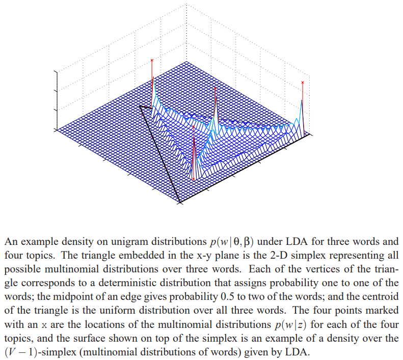
As shown in the LDA paper, the distribution of \(\mu\) is a continuous mixture with a Dirichlet prior \(p(\theta|\alpha)\) as mixture weights, hence the pdf exhibits a multimodal structure when \(\alpha<1\). It can also be acquired by applying a change of variable to the prior pdf \[p(\mu|\alpha,\beta) = p(f_\beta(\theta)|\alpha).\] When \(\mu\) is of greater dimensions than \(\theta\) it actually lives on a subspace of the simplex, where the bases are the rows of \(\beta\) (topics).

Training and Inference

Variational inference + expectation-maximization
In the LDA model described above, \(\theta\) and \(z\) are latent variables, \(\alpha\) and \(\beta\) are parameters.

This paper David M Blei, Andrew Y Ng, and Michael I Jordan. Latent dirichlet allocation. 2003. shows how to use expectation-maximization (EM) for a maximum likelihood estimation (MLE) of the parameters \(\alpha\) and \(\beta\). The main problem is, the distribution of latent variables \(p(\theta,\mathbf{z}|\mathbf{w},\alpha,\beta)\) is intractable to compute, a nice approximation method based on variational inference was given in the paper.

Since MLE looks for high likelihood, there’s an inclination towards sparse \(\alpha\) and \(\beta\).

Collapsed Gibbs sampling
A common extension of the original LDA model is to model \(\beta\) as a latent variable with another Dirichlet distribution \(p(\eta)\) as its prior. Then by treating \(\alpha\) and \(\eta\) as hyper-parameters, this paper Thomas L Griffiths and Mark Steyvers. Finding scientific topics. 2004. uses collapsed Gibbs sampling to sample directly from the posterior \(p(\mathbf{z}|\mathbf{w})\) instead of doing an optimization.

The training procedure (convergence/burn-in of Markov chains) can be shown as minimizing the KL divergence between the initial distribution and the equilibrium via the transition (see Section 4.4 of Elements of Information Theory (Second Edition) and this tutorial) \[z_i^{(t+1)}\sim p(z_i|\mathbf{z_{\backslash i}^{(t)}}).\] In the collapsed Gibbs setting, it turns out the only information necessary for sampling from \(p(\mathbf{z}|\mathbf{w})\) are the document–topic counts \(n_m\) and the topic–term counts \(n_k\), which allows the algorithm to be implemented efficiently.

Based on a full set of samples \(\mathbf{z}\), the distribution of \(\beta\) and \(\theta\) can be estimated by \[p(\theta|\mathbf{w},\mathbf{z},\alpha) = Dir(\theta|n_m+\alpha)\] \[p(\beta|\mathbf{w},\mathbf{z},\eta) = Dir(\beta|n_k+\eta)\] For inference, collapsed Gibbs sampling can also be used to sample the latent variable \(\tilde{\mathbf{z}}\)
\[p(\tilde{\mathbf{z}}|\tilde{\mathbf{w}},\mathbf{z},\mathbf{w})\] see Parameter estimation for text analysis for details.

Dontloo's Blog